Seismic Refraction Introduction.

Classical Seismic Refraction

Reading Resources

• CH 6 Seismic Refraction from LITE.

• CH 2 Seismic Exploration - Fundamental Considerations from I2AG.

  • Image files: JPGs in a ZIP file

• CH 3 Seismic Exploration - The Refraction Method from I2AG

  • Image files: JPGs in a ZIP file

The Seismic Sprint

Note that what is shown in the animation relies on:

• The seismic velocity of the lower layer is larger than the upper layer, i.e. $V_2>V_1$$V_2 > V_1$.

• There is a critical angle of incidence, ${\theta }_{ic}$$\theta_{ic}$, for which the refraction angle is 90 degrees.

In the video, the data is plotted as distance vs. time, so the slopes are already in units of $\frac{m}{s}$$\frac{m}{s}$.

However, almost always you will see this type of data plotted as time vs. distance, so that the slopes are in units of $\frac{s}{m}=\frac{1}{V}$$\frac{s}{m}=\frac{1}{V}$ (i.e. reciprocal of velocity). This is because when you have multiple slope breaks on a plot of first-arrivals, it is easier to plot is as increasingly shallower slopes rather than increasingly larger slopes. But, as you know, this is an arbitrary convention.

However you plot the data, such a plot is referred to in various ways:

• first-break plot

• first-arrival plot

• travel-time curve of the first arrivals/breaks.

Confusing, eh?

Wave names

Note that the video shows many distinct names of the waves along the raypaths:

• Direct wave

• Critically refracted wave

• Head waves

  • When we were at Brizziolari Creek I didn't use the term head wave and just referred to that as part of the critically refracted wave (to reduce terminology at the moment).

General Behavior of a wave (or raypath) at a boundary

In the above video we only saw the refracted wave that is the critically refracted wave. But the wave has a wavefront, meaning that wave energy reaches the boundary at all angles - not just the critical angle. So what happens in the general case where the angle of incidence on the boundary, ${\theta }_1$$\theta_1$, is not the critical angle of incidence, ${\theta }_{ic}$$\theta_{ic}$?

This is encapsulated in Snell's Law: $\frac{sin({\theta }_1)}{V_1}=\frac{sin({\theta }_2)}{V_2}$$\frac{sin(\theta_1)}{V_1} = \frac{sin(\theta_2)}{V_2}$

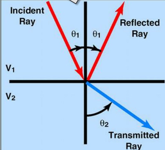
Figure 1. Illustration of the typical case for reflected and transmitted (or, refracted) waves as a boundary.

Question: In Figure 1 just above, it is implied that $V_2>V_1$$V_2 > V_1$. How would the way the image is drawn change if $V_2<V_1$$V_2 < V_1$?

Please watch the linked to animated video. It shows the idea of a wavefront, rather than just single raypaths, as well as all the cases of incidence angle at a boundary. $si{n}^{-1}(\theta )$$sin^{-1}(\theta)$

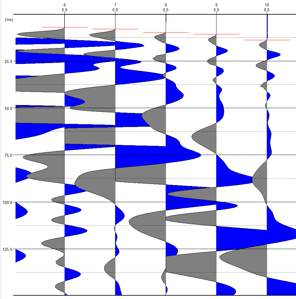
Figure 2. P-wave first break or first arrival times. The first-break times are marked by a red linew at each geophone. Wave arrivals following this are various types of reflected and refracted waves, from even deeper boundaries than the first boundary.

All the complexity of wave arrivals following the first break (Figure 2) are not needed in classic seismic refraction is not needed - all we use are the first-break (or, first-arrival) times, i.e. the time of the red bar (in figure above) at each geophone distance. But other seismic methods do use the later arriving waves. The complexity of the "wave-field" is whatmakes seismology difficult, but, if you are so inclined, also interesting.

Plotting First-arrival Data

If you are using a spreadsheet to plot your first-arrival data in your reports, you will want to make it look something like Figure 3:

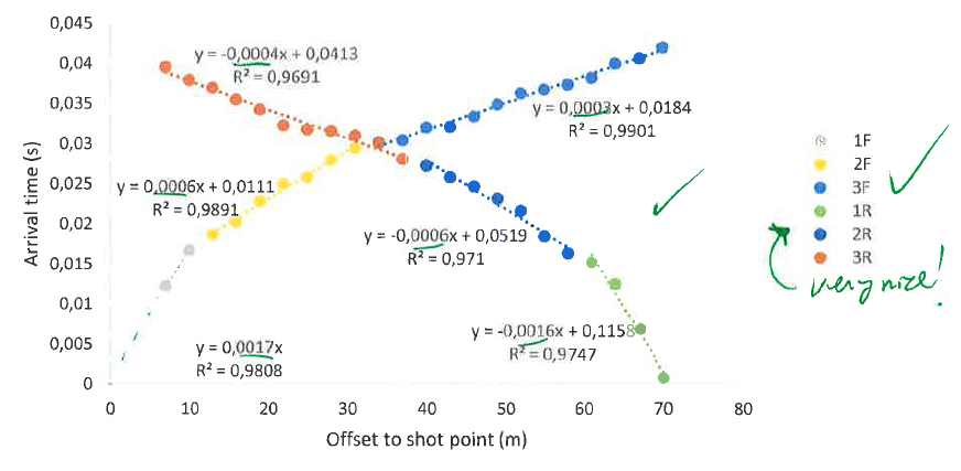
Figure 3. Example plot of "forward" and "reverse" first-break data. Arrival times (dots) are grouped together between slope breaks and the best linear-fit is displayed for each group along with the R-squared measure of fit value.

Back to the GEOL 420 Homepage