Practice Questions

i.e. "homework" - but not collected. Like eating your vegetables, it's good for you to ingest. Aside from those problems listed here, there are also problems in the chapter readings that are provided with each topic - you should take a look at those that are related to our class discussions.

General advice: Use more illustrations than words. Make annotated sketches. The groups below are arbitrary, they just mean that I put them into the list at the same time.

Group 1

1. Illustrate how geometry affects the resistance of a geologic, or other, material like a copper wire.

2. How would you communicate the difference between resistance and resistivity?

3. Why do we want to do resistivity geophysical surveys, rather than resistance surveys?

4. What concepts from circuits does Ohm's Law relate? What are the units of all the variables? Can you describe in simple terms what each of them means?

5. What is the geometric idea for converting between resistance and resistivity? Illustrate it, and also write down the general formula.

6. Illustrate how to make a single resistivity measurement using four electrodes and common spacing. What is the name of this type of geometry? What is the formula for the geometric factor in the case of this geometry, or array, style? What does the geometric factor do?

7. How would you interpret the phrase resistance equals an integrated value of resistivity? It's not a precise phrase - a sketch may help you parse it.

Group 2

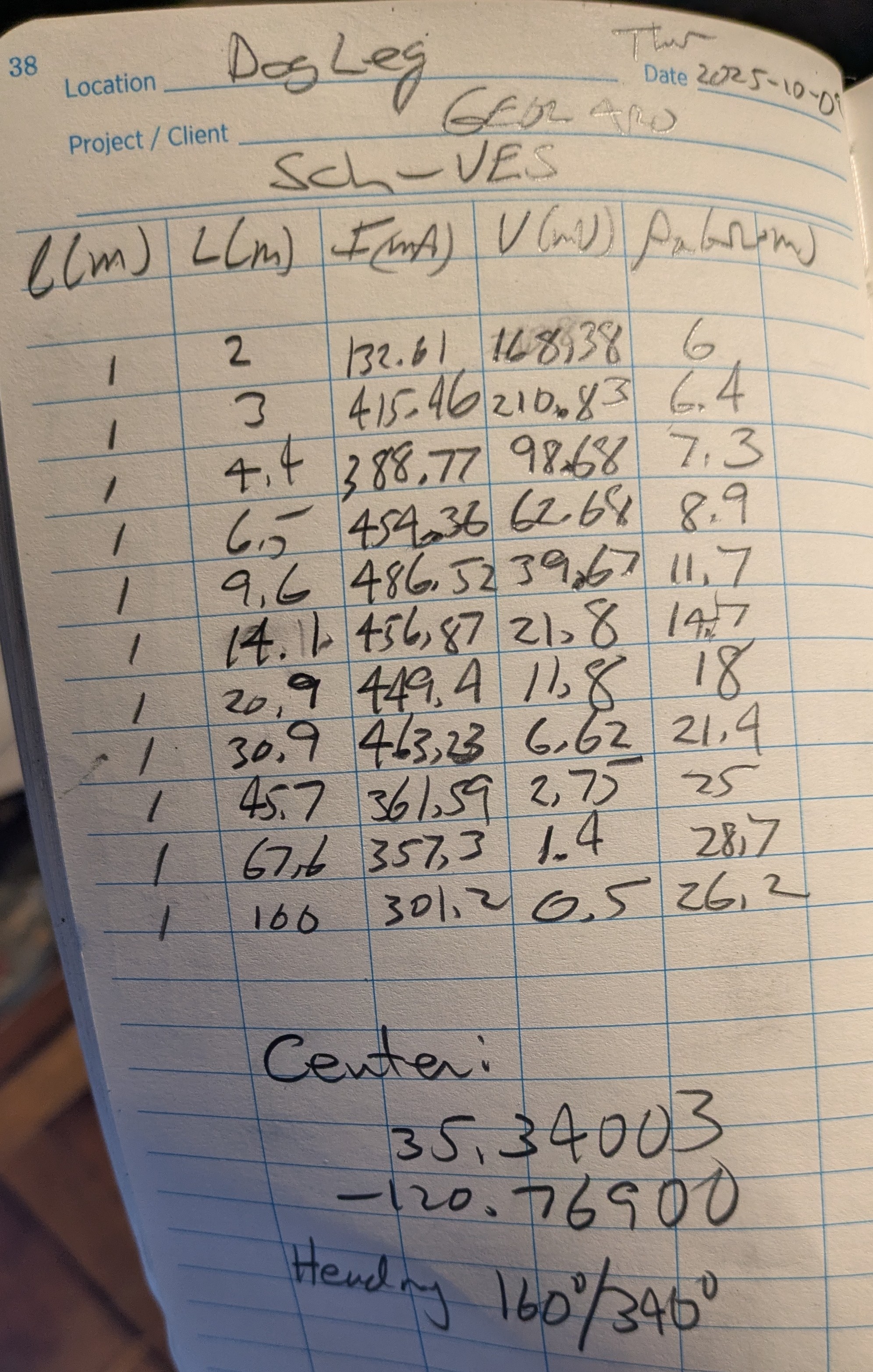
8. You have VES data for a profile on which a Schlumberger and Wenner style were collected at the Dog Leg, near our Wenner VES profile. Also here are the Schlumberger field notes and Wenner field notes. For each data set:

• Read the data into RES1D

• Invert the data for a subsurface model of electrical resistivity

• Group layers together to make a simpler (less layers) model

• Compare the two models - are they materially different? What can you conclude?

8. I emailed you an Overleaf template for our reports. Make an additional copy of it in your Overleaf account and modify it with your own image files and words to learn how to use Overleaf to make a simple report. In particular, there are some links in there to show you how to make a table - make one! Some of you have experience using Overleaf/LaTeX before, others not. Consult one another, the mighty internet, and of course me. Make sure you can do this - it is required you submit your reports in the course using Overleaf.

9. Make a sketch of how an energetic young field crew (i.e. the Cuyama Valley SuperStingers) could use VES and CST to build up a systematic set of image points in two dimensions in the subsurface

10. Learn how to use RES1D to carry out forward modeling - I will describe in class and then post some activities here.

• Activities:

  • How thin of a layer that is low-resistivity sandwiched between two layers of higher resistivity can you "see" with a Wenner VES? What is the shape of the apparent resistivity data? What if the intermediate layer is higher resistivity than the surrounding layers?

  • In general, given a set of flat layers of various thicknesses and constant resistivity, can you predict the shape of the apparent resistivity curve?

11. Examine these Schlumberger field notes, which includes the field measurements of current, I, and voltage, V. However, the operator made a mistake in setting up the "l" parameter into the resistivity meter for data collection. In the notes it says $l=1$$l = 1$ , and this is what was input into the resistivity meter. After the collection was over, during cleanup it was noticed that instead $l=2$$l = 2$ . Therefore the values of apparent resistivity computed by the resistivity meter, and noted in the field notes, are wrong. Can you fix them?

12. See if you can make sense of this case study: Time-domain electromagnetic soundings to characterize water quality within a fresh-water-saline-water transition zone, Estancia Valley, New Mexico done by the US Geological Survey in 2005 (color printed copies are in the geology classroom in the back corner by the large wall map). Don't be afraid of the "time-domain electromagnetic sounding" phrase in the title. This is just another method to collect the same resistivity parameter we have been talking about - except the method of collection is different. The term "sounding" still means it is a one-dimensional data set. The advantage of this other method (Figure 4) is that you can get your data points to be much deeper. If you move around your sounding point, you can make a pseudo-profile.

• Try to connect the resistivity sounding data to the geologic structures that are summarized (Figures 3, 7). Are the folded sedimentary units shown in Figure 3 seen in the resistivity data of Figure 7?

• How would you summarize the results? Does the geophysical/resistivity data support the geologic observations? Is the resistivity too low in resolution to make you confident about their conclusions?

Group 3

• In your reading (the one I passed out to you but is also posted) there is a discussion of the "equivalence principle". Use REDS1D to illustrate this principle by making two models for comparison of forward modeling and inverse modeling of the forward modeling.

• The Lockshaw Ranch webpage contains links to articles, includding Lachassagne et al., 2011, Dewandel et al., 2006, and Belle et al., 2018. The latter two papers discuss the laminated layer, while Lachassagne et al., 2011 lays out a conceptual model of granitic hardrock aquifers controlled by weathering and biotite swelling. Be prepared to briefly discuss the primary ideas of these articles using annotated sketches and short amounts of text.

  • What is the conceptual model? What is the laminated layer? What is its role in citing permeable fractured granite? What resistivity is thought to represent permeable fractured granite? What resistivity represents the unweathered/competent granite? How does any of this compare the the data we have at Lockshaw Ranch?

Group 4

• Run a systematic set of Survey Planner tests to help build intuition about how resolution, "blurring", inversion artifacts, etc work. Start simple and add one piece of complexity at a time. Adding too much at once will not allow you to build the intuition you want.

  • You might think about making progressively complex models mimicking what you think is going on at the Dog Leg.

Group 5

• What are the mechanisms of electrical conduction in rocks and geologic materials? Using the reading materials below, add to your "Field Report 2 Appendix" assignment with a description of the how electricity is conducted in rocks.

  • Reading 1 from I2AG.

  • Reading 2 - NYL from Geophysics for the Mineral Exploration Geoscientist.

Group 6 Seismic Refraction

• At Brizziolari Creek we obtained a 1.9-meter thick top layer with a P-wave velocity of ~ $360\frac{m}{s}$$360 \frac{m}{s}$, and a lower layer velocity of ~ $2,000\frac{m}{s}$$2,000 \frac{m}{s}$. The shot offset was also 1-meter. Calculate:

  • The critical angle of incidence on the boundary, ${\theta }_{ic}$$\theta_{ic}$.

  • The critical distance $x_{crit}$$x_{crit}$.

  • The crossover distance $x_{co}$$x_{co}$.

  • Make a sketch the illustrates the entire scenario.

• Do the same as above, except imagine a deeper system where the first layer has a thickness of 50 meters and velocity of $1,000\frac{m}{s}$$1,000 \frac{m}{s}$ and the lower layer velocity is $3,000\frac{m}{s}$$3,000 \frac{m}{s}$. Imagine you have all the profile length and geophones you need for the seismic refraction survey.

  • As a follow up, about how long would your profile need to be to detect the contact in the above scenario?

• You just used the "30%" rule of thumb in the question above. Derive this rule of thumb. In other words, why is it that the deepest interface a seismic refraction survey can detect, if one exists there, is about 30% of the profile length? This is a more challenging problem but very instructive.

• From the "LITE" book chapter on refraction seismology CH 6, do problems 5, 7, and 8.

• From the "I2AG" book chapter on refraction seismology CH 3, do problems 3.2, 3.4, 3.6, 3.7, 3.8, 3.11, 3.13

• In the "I2AG" book chapter on refraction seismology CH 3 read about the non-ideal subsurface called a "low-velocity layer".

  • If you have a three-layer system but the middle layer is of lower velocity than the layer above (and, also lower than the layer below) illustrate why the data will only look like a two layer system How does Snell's Law factor into this?

  • From your data, you will see only one slope break, and so you could calculate the thickness of a top layer. But, to which actual interface in the subsurface (there are two, after all) does the calculated thickness correspond - the first, the second? And is the calculated depth correct? If not, is the under- or over-estimated? Illustrate how you reasoned this out. Using a quantitative example of the above situation of your own making would be useful, too.

That's all for now ... stay tuned for more fun 😉 

Back to the GEOL 4420 Homepage